It looks like a spilling paint bucket. I feel certain that Microsoft will continue to complete this work over.
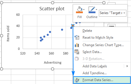
Find Label And Highlight A Certain Data Point In Excel Scatter Graph Ablebits Com
This will open the Format Task Pane with Chart Options selected.
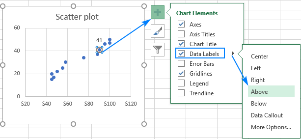
. You should see the Format Object Task Pane on the right-hand side of the Excel window. Click green plus data labels center click green plus double click in chart label contains click percentage click values check box click close click home font 18. For newer charts the pane is there but its blank.
To format data labels Step 1 Right-click the data label and then click Format Data Label. Then select the data labels to format from the Current Selection button group. This is what I want.
Use the Format Data Labels task pane to display Percentage data labels and remove the Value data labels. As of today in the Insider Fast builds the Format Data Series task pane is operational for older charts. Theres also a feature called data callouts which wraps data labels in a shape.
2 Right click on the data label and then choose Format Data Label. Use the Format Data Labels task pane to display Percentage data labels and remove the Value data labels. The Pane - Format Data Label format appears.
One way to do this is to click the Format tab within the Chart Tools contextual tab in the Ribbon. Right click on one of the data series bars in the chart. Either of these options opens the Format Data Labels Task Pane as shown in Figure 3 below.
Elements and Options Of Chart in Excel - DataFlair. This work is now going on. This will then cause Word to display the contextual Chart Tools Design and Format tabs.
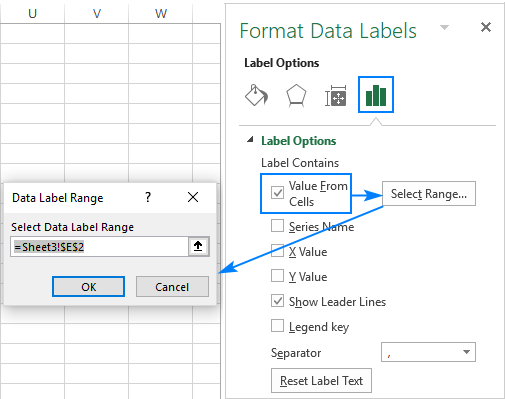
Format Data Labels option. You can set data labels to show the category name the series name and even values from cells. Replied on April 6 2021.
Apply 18 point size to the data labels. The styles are displayed formatted as they are defined. To format data labels select your chart and then in the Chart Design tab click Add Chart Element Data Labels More Data Label Options.
In the task pane click the Fill. When other editors in my group open a document they have to access the Styles pane from the Home ribbon Styles area. Next set the labels DataLabelBaseShowValue property or any other DataLabelBaseShow property depending on the information you wish to display in the label to true.
Use Insert Illustrations Chart to choose the chart type. Format Data Labels in Excel. Excel displays the Format Data Series task pane at the right side of the chart.
In this case for example I can. Excel displays a Context menu. Next select the Series Options button to display the Series Options and Color choices.
Choose Format Data Series from the Context menu. The short story is that because of the change Microsoft has to re-work the interface. These two tabs provide you with all chart data label formatting options.
Step 3 Under FILL click Solid Fill and select a color. A T-chart however is more like a table and for that a table is more appropriate. Apply 18 point size to the data labels.
The easiest way to display the Format Task Pane is to double-click on a chart. Alternatively the user can also click More Options in data labels options to display on the format data label task pane. From this menu choose the Format Data Labels option.
If the Series Options arent already displayed then click the Series Option expander button on the right side and select the Series value option that corresponds with your data. Step 2 Click the Fill icon and line icon. Close the task pane.
Up to 24 cash back emphasis etc. Fill and Line options appear below it. I dont remember what I did years ago to get this version of the Styles pane to show.
Close the task pane. In this Task Pane youll find the Label Options and Text Options tabs. You can also select a chart element first then use the keyboard shortcut Control 1.
To make data labels easier to read you can move them inside the data points or even outside of the chart. You wont be able to format the chart until after you have inserted it. When first enabled data labels will show only values but the Label Options area in the format task pane offers many other settings.
Click Label Options and under Label Contains pick the options you want. To format data labels in Excel choose the set of data labels to format. Click green plus data labels center click green plus double click in chart label contains click percentage click values check box click close click home font 18.
What they see is a floating window with an unformatted list of. To display an individual data label add a DataLabel instance to the DataLabelCollection collection with the index set to the index of the selected data point.
Find Label And Highlight A Certain Data Point In Excel Scatter Graph Ablebits Com
Find Label And Highlight A Certain Data Point In Excel Scatter Graph Ablebits Com

Formatting Data Labels And Printing Pie Charts On Excel For Mac 2019 Microsoft Community

Find Label And Highlight A Certain Data Point In Excel Scatter Graph Ablebits Com


0 Comments